School of Economics

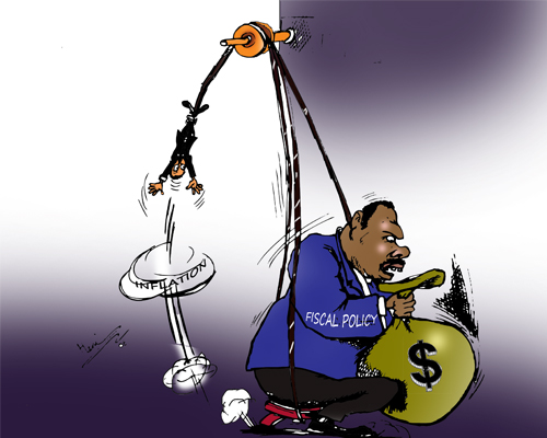
Fiscal Policy

Fiscal policy

3-6-17

Fiscal policy: Congress action to control government changes in the expenditures or tax revenues of federal government

2 tools of fiscal policy

1. Taxes - government can increase or decrease taxes
2. Spending - government can increase or decrease spending

Fiscal policy was enacted to promote our nation's economic goals: full employment, price stability, economic growth

Deficits, surpluses, budgets

• Balanced budget: revenues = expenditures
• Budget deficit: revenue < expenditures
• Budget surplus: revenues > expenditures

Government debt: sum of all deficits - sum of all surpluses

Government borrows money from:

1. Individuals
2. Corporations
3. financial institutions
4. foreign entities or governments

Options of fiscal policy

1. Discretionary fiscal policy (think deficit)
2. Contractionary fiscal policy (think Surplus)
3. non-discretionary fiscal policy (no action)

Three types of taxes

1. Progressive taxes are taxes that take larger percent of income from high-income groups
2. Proportional taxes or flat rates take some percent of income from all income groups
3. Regressive taxes text larger percent from low-income groups

Contractionary fiscal policy (the brake)

• Laws that reduce inflation, decrease GDP (close inflation gap)
• Government spending decrease
• tax increase
• Combination of the two

Expansionary fiscal policy (the gas)

• Laws that reduce unemployment and increase GDP (close recession gap)
• Increase government spending
• decrease taxes

Automatic / built-in stabilizers

• Anything that increases government budget deficit during a recession and increases its budget surplus during inflation without requiring explicit action by policy makers

Multipliers

Multipliers

2-24-17

The spending multiplier effect: An initial change in spending (C, Ig, G, Xn) causes larger change in AS or AD

• Formula for multiplier: change in AD/ change in spending OR change in AD/ change in C, Ig, G, or Xn
• This happens because expenditures and income flow continuously which sets off a spending increase in economy

Calculating spending multiplier

• Formula: 1/ 1- MPC OR 1/MPS

Calculating tax multiplier

• When government taxes, the multiplier works in reverse because now money is leaving circular flow
• Tax multiplier formula: -MPC/1-MPS OR -MPC/MPS
• If tax is cut, multiplier is positive because now more money in circular flow

Consumption and Saving

Consumption and Saving

2-23-17

Disposable Income (DI) - income after taxes or net income

• DI= gross income - taxes

With DI Households can either

1. Consume
2. Save

Consumption:

• Household spending
• Ability to consume is constrained by:
• Amount of DI
• Propensity to save
• Households consume if DI = 0, because of credit cards and checks (autonomous consumption). This is Dissaving.
• APC (average propensity to save) = C/DI (% DI that is spent)

Savings:

• Household not spending
• Saving is constrained by:
• Amount of DI
• Propensity to consume
• Households do not save when DI = 0
• APS (average propensity to save) = S/DI (% DI not spent)

Formulas

• APC + APS = 1
• 1 - APC = APS
• 1 - APS = APC

APC > 1 = Dis-saving

-APS = Dis-saving

MPC and MPS

• Marginal propensity to consume
• Change in C / change in DI
• % of every extra dollar earned that is spent

• Marginal propensity to save
• Change in S / Change in DI
• % of every extra dollar earned that is saved

**DI = disposable income, C = consumption**

Formulas

• MPC + MPS = 1
• 1 - MPC = MPS
• 1 - MPS = MPC

Determinants of consumption and savings

• Wealth
• Expectations
• Household Debt
• Taxes

Aggregate Supply

Aggregate Supply

2-21-17

Aggregate Supply: Level of real GDP firms will produce at each price level.

Long and Short Run

• Long run: Period of time where input prices are completely flexible and adjust to changes in price level
• Level of real GDP supplied is independent of price level
• Short run: Period of time where input prices are sticky and do not adjust to changes in the price level.
• Level of real GDP supplied is directly related to the price level

Long Run Aggregate Supply (LRAS)

• The long run aggregate supply marks the level of full employment in the economy (analogous to PPC)

Short Run Aggregate Supply (SRAS)

• Because input prices are sticky in the short run, SRAS is upward sloping.
• Key to shifts in SRAS is per unit cost of production
• Per-unit production cost: total input cost/ total output
• Changes in SRAS:
• Input Prices
• Productivity
• Legal-Institutional environment

Interest Rates and Investment Demand

Interest Rates and Investment Demand

2-21-17

Investment: What we want to spend $ on

• Money spent on:
1. New Plants (factories)
2. Capital equipment (machinery)
3. Technology (hardware / software)
4. New homes
5. Inventories (goods sold by producers)

Expected Rates of Return

• Business makes investment sections with cost/benefit analysis.
• Business determine the benefits with expected rate of return
• Business counts the cost with interest costs.
• Business determines amount of investment they undertake by:
• Comparing expected rate of return to interest cost.
• If expected return is > interest cost, then invest
• If <, don't invest

Real (r%) and Nominal (i%)

• Formula : r% = i% - Inflation
• Nominal is observable rate of interest. Reseal subtracts out inflation and is ex post facto.
• Real interest rate determines cost of investment decision
• Investment Demand Curve (ID) is downward sloping
• Shifts in ID
• Cost of production
• Technology change
• Business taxes
• Stock of capital
• Expectations

Aggregate Demand

Aggregate Demand

2-16-17

Aggregate Demand: Demand by consumers, businesses, govt, and foreign countries.

• Changes in price level cause a move along curve not a shift.
• AD = C + IG + G + Xn

*inverse relationship between price level and real GDP.*

Why is AD downward slipping?

1. Wealth Effect

• higher price reduce purchasing power of $
• decreased quantity of expenditures
• Lower price levels increase purchasing power and increase expenditures.

2. Interest rate Effect

• As price level rises, lenders need to charge higher interest rates to get real return of rates

3. Foreign Trade Effect

• When U.S price level increases, foreign buyers buy less U.S goods, Americans buy more foreign.
• Exports fall, imports rise real GDP demanded to fall.

4 Determinants of AD

1. Consumption
2. Gross Private Domestic Investment
3. Government Spending
4. Net Exports (Exports-Imports)
• AD increase shift  →
• AD decrease shift ←
• More govt spending AD →
• Less govt spending AD ←
• AD = GDP = C+Ig+G+Xn